Closed-Form Math for Multi-Hop Arbitrage: Folding N Constant-Product Pools in Microseconds

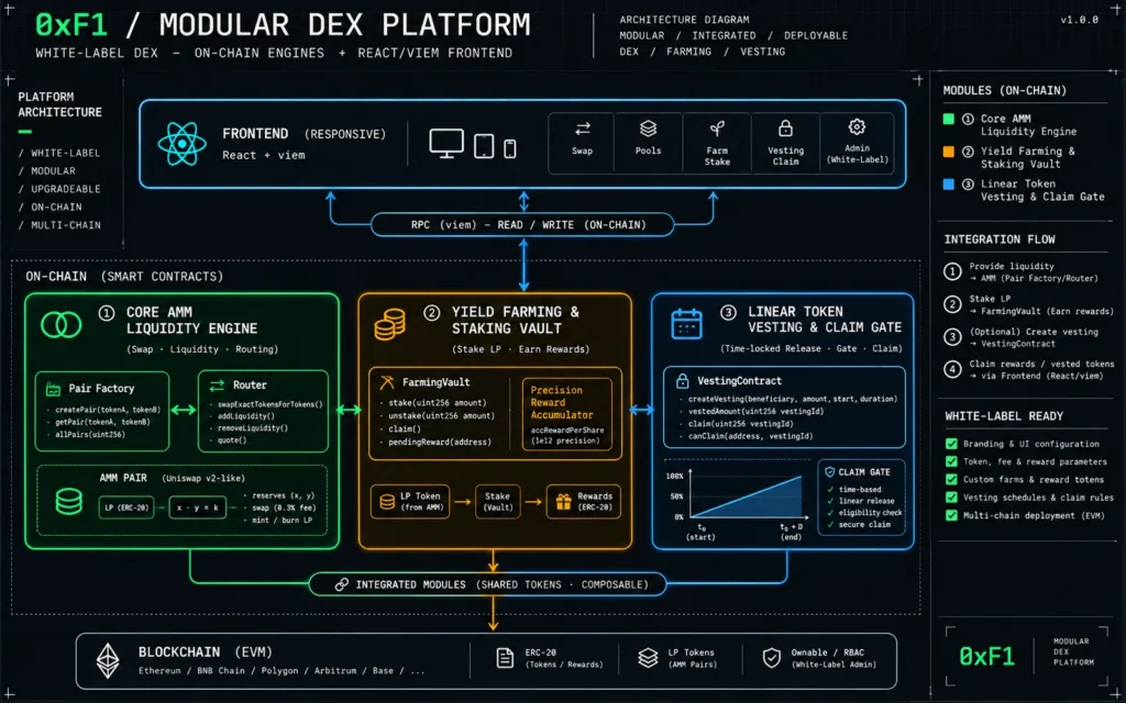
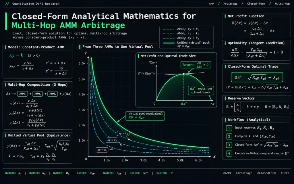
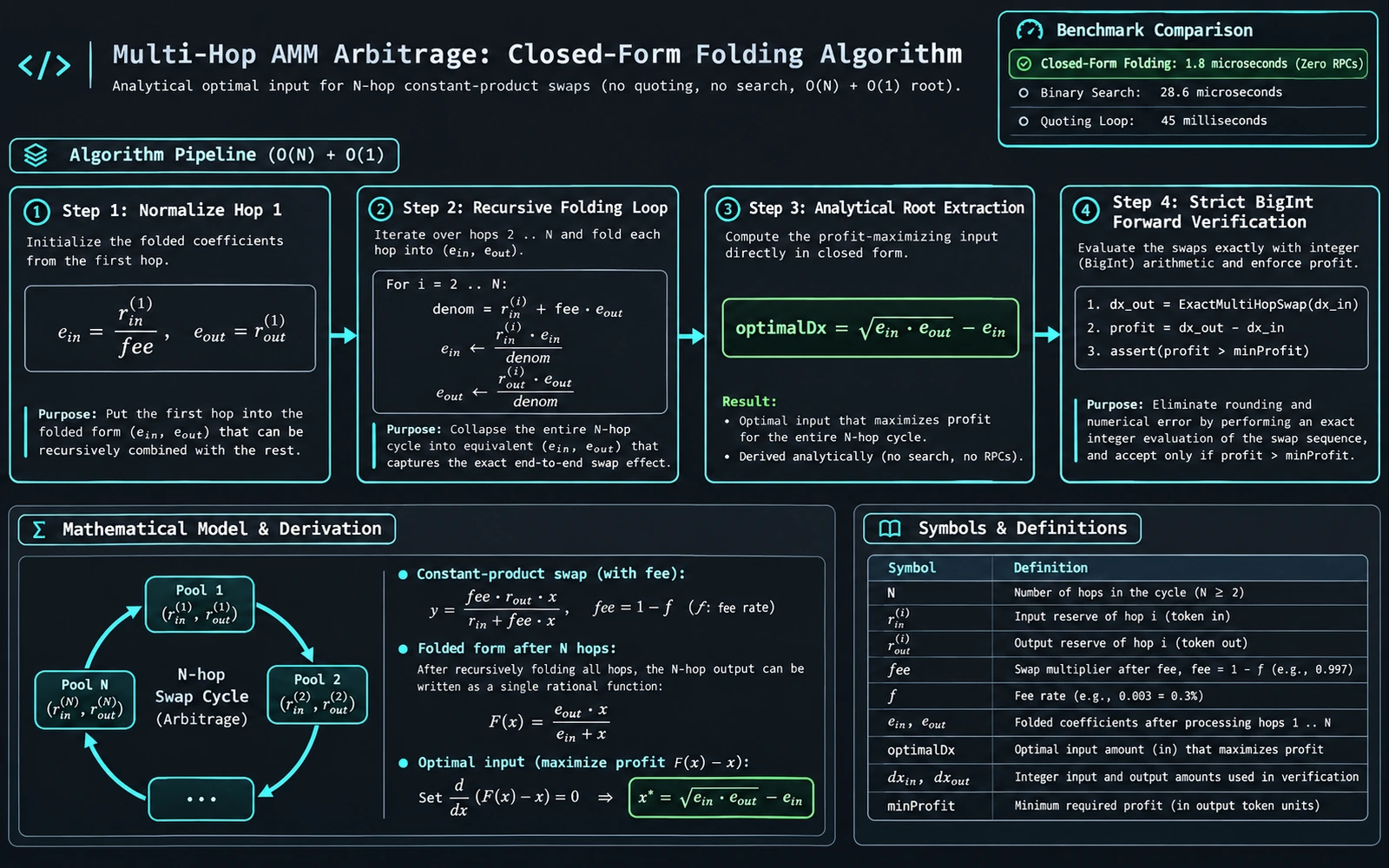
In competitive EVM on-chain arbitrage, numerical approximation methods (such as binary or ternary search) introduce prohibitive CPU and RPC latency into the execution pipeline. Evaluating optimal borrow amounts across 2-hop spatial routes or 3-hop triangular cycles (WETH -> USDC -> TOKEN -> WETH) requires solving an analytical optimization problem in microseconds. In White-Label DEX Launch Kit and our EVM execution engine, this is achieved by recursively folding N constant-product pools into a single virtual pool (E_in, E_out), extracting the exact global derivative maximizer in closed form, and validating the output through a zero-drift BigInt forward verification pass.

1. The Latency Trap: Why Numerical Search Fails in High-Frequency MEV

When an automated liquidity event occurs (for example, a Uniswap V2 or Aerodrome pair emitting a Sync log indicating a whale swap), the price ratio between token pairs shifts temporarily, creating an arbitrage opportunity.

To capitalize on this price discrepancy via flash loans, an execution bot must calculate the input amount Δx^* that maximizes net profit:

Π(Δx) = y_N(Δx) − Δx

where y_N(Δx) represents the token output received after executing swaps across N sequential liquidity pools.

Many developers resort to iterative numerical algorithms:

• Binary Search / Bisection: Evaluates midpoint derivatives iteratively. Requires 15 to 30 iterations to achieve sufficient integer precision, costing between 5 to 25 milliseconds of CPU time per route.
• RPC Quoting Loops: Querying node endpoints via quoteExactInput or getAmountsOut over JSON-RPC. Each network round-trip adds 15 to 60 milliseconds. By the time the search converges, competing searchers on the block sequencer have already backrun the transaction.

To compete at the sub-millisecond level, the solver must evaluate the optimal input analytically in memory. While closed-form solutions for 2-hop arbitrage are well known, production triangular and multi-hop cycles require generalizing this solution to an arbitrary number of interconnected pools.

2. Mathematical Derivation: Recursive Virtual Pool Folding

Consider an individual Uniswap V2 constant-product pool with input reserve R_in, output reserve R_out, and fee factor γ ∈ (0, 1] (where γ = 0.997 for standard 0.3% fee pools, or 0.9970 with 10, 000 base scaling).

The output amount y for a given input x is defined by the standard AMM formula:

$$y(x) = \frac{\gamma \cdot R_{\text{out}} \cdot x}{R_{\text{in}} + \gamma \cdot x}$$

Dividing both numerator and denominator by γ, we can express the swap function in canonical homographic form:

$$y(x) = \frac{R_{\text{out}} \cdot x}{\frac{R_{\text{in}}}{\gamma} + x}$$

We define the Initial Virtual Reserves for the first hop (k = 1):

$$E_{\text{in}}^{(1)} = \frac{R_{\text{in}, 1}}{\gamma_1}, \quad E_{\text{out}}^{(1)} = R_{\text{out}, 1}$$

The output of hop 1 is thus:

$$y_1(x) = \frac{E_{\text{out}}^{(1)} \cdot x}{E_{\text{in}}^{(1)} + x}$$

Recursive Composition Across Hop k

Now, suppose the output y₁ is fed directly into a second pool (k = 2) with reserves (R_in, 2, R_out, 2) and fee factor γ₂:

$$y_2(x) = \frac{R_{\text{out}, 2} \cdot y_1}{\frac{R_{\text{in}, 2}}{\gamma_2} + y_1}$$

Substituting $y_1(x) = \frac{E_{\text{out}} \cdot x}{E_{\text{in}} + x}$:

$$y_2(x) = \frac{R_{\text{out}, 2} \left( \frac{E_{\text{out}} \cdot x}{E_{\text{in}} + x} \right)}{\frac{R_{\text{in}, 2}}{\gamma_2} + \left( \frac{E_{\text{out}} \cdot x}{E_{\text{in}} + x} \right)}$$

Multiplying numerator and denominator by (E_in + x):

$$y_2(x) = \frac{R_{\text{out}, 2} \cdot E_{\text{out}} \cdot x}{\frac{R_{\text{in}, 2}}{\gamma_2}(E_{\text{in}} + x) + E_{\text{out}} \cdot x} = \frac{R_{\text{out}, 2} \cdot E_{\text{out}} \cdot x}{\frac{R_{\text{in}, 2}}{\gamma_2} \cdot E_{\text{in}} + \left( \frac{R_{\text{in}, 2}}{\gamma_2} + E_{\text{out}} \right) x}$$

Multiplying numerator and denominator by γ₂:

$$y_2(x) = \frac{\gamma_2 \cdot R_{\text{out}, 2} \cdot E_{\text{out}} \cdot x}{R_{\text{in}, 2} \cdot E_{\text{in}} + (R_{\text{in}, 2} + \gamma_2 \cdot E_{\text{out}}) x}$$

To restore this equation back to the canonical single-pool form $y(x) = \frac{E_{\text{out}}' \cdot x}{E_{\text{in}}' + x}$, we divide both numerator and denominator by the coefficient of x, namely (R_in, 2 + γ₂ ⋅ E_out):

$$E_{\text{in}}' = \frac{E_{\text{in}} \cdot R_{\text{in}, 2}}{R_{\text{in}, 2} + \gamma_2 \cdot E_{\text{out}}}$$

$$E_{\text{out}}' = \frac{\gamma_2 \cdot E_{\text{out}} \cdot R_{\text{out}, 2}}{R_{\text{in}, 2} + \gamma_2 \cdot E_{\text{out}}}$$

General Folding Theorem for N Pools

By induction, any sequence of N constant-product pools chained together collapses into a single virtual pool parameterized by (E_in, E_out):

$$y_N(x) = \frac{E_{\text{out}} \cdot x}{E_{\text{in}} + x}$$

where E_in and E_out are computed iteratively using:

denom_k = R_in, k + γ_k ⋅ E_out^{(k − 1)}

$$E_{\text{in}}^{(k)} = \frac{E_{\text{in}}^{(k-1)} \cdot R_{\text{in}, k}}{\text{denom}_k}$$

$$E_{\text{out}}^{(k)} = \frac{\gamma_k \cdot E_{\text{out}}^{(k-1)} \cdot R_{\text{out}, k}}{\text{denom}_k}$$

Extracting the Analytical Root

The net arbitrage profit function is:

$$\Pi(x) = y_N(x) - x = \frac{E_{\text{out}} \cdot x}{E_{\text{in}} + x} - x$$

Taking the first derivative with respect to x and setting it to zero:

$$\frac{d\Pi}{dx} = \frac{E_{\text{out}} \cdot E_{\text{in}}}{(E_{\text{in}} + x)^2} - 1 = 0$$

(E_in + x)² = E_in ⋅ E_out

$$E_{\text{in}} + x = \sqrt{E_{\text{in}} \cdot E_{\text{out}}}$$

Solving for x:

$$\Delta x^* = \sqrt{E_{\text{in}} \cdot E_{\text{out}}} - E_{\text{in}}$$

Condition for Existence of Arbitrage: A profitable arbitrage opportunity exists if and only if: Δx^* > 0 ⇔ E_out > E_in If E_out ≤ E_in, the effective price product across the route does not overcome the compounded fee drag, and the solver terminates immediately with zero overhead.

3. Production TypeScript Implementation

In evm-arbitrage/resident-bot.ts:L202-L244, this derivation is implemented in production code:

export interface PoolHopReserve {
  rIn: bigint;
  rOut: bigint;
  feeBps: bigint; // Supports 997 (per-thousand) or 9970 (per-ten-thousand)
}

export class ArbitrageMath {
  public static solveOptimalMultiHop(
    hops: PoolHopReserve[]
  ): { optimalInput: bigint; expectedProfit: bigint } {
    if (hops.length < 2) return { optimalInput: 0n, expectedProfit: 0n };

    // 1. Normalize initial hop into a canonical virtual pool (eIn, eOut)
    const firstScale = hops[0].feeBps > 1000n ? 10000 : 1000;
    const firstFee = Number(hops[0].feeBps) / firstScale;
    let eIn = Number(hops[0].rIn) / firstFee;
    let eOut = Number(hops[0].rOut);
    if (eIn <= 0 || eOut <= 0) return { optimalInput: 0n, expectedProfit: 0n };

    // 2. Recursively fold subsequent hops into the equivalent virtual pool
    for (let i = 1; i < hops.length; i++) {
      const rInNext = Number(hops[i].rIn);
      const rOutNext = Number(hops[i].rOut);
      const scaleNext = hops[i].feeBps > 1000n ? 10000 : 1000;
      const fNext = Number(hops[i].feeBps) / scaleNext;
      if (rInNext <= 0 || rOutNext <= 0 || fNext <= 0) return { optimalInput: 0n, expectedProfit: 0n };

      const denom = rInNext + fNext * eOut;
      eIn = (eIn * rInNext) / denom;
      eOut = (eOut * rOutNext * fNext) / denom;
    }

    // Terminate if compounded rate does not cover cumulative fees
    if (eOut <= eIn) return { optimalInput: 0n, expectedProfit: 0n };

    // 3. Analytical first-derivative root of the folded virtual pool
    const optimalDxFloat = Math.sqrt(eIn * eOut) - eIn;
    if (optimalDxFloat <= 0) return { optimalInput: 0n, expectedProfit: 0n };

    const dx = BigInt(Math.floor(optimalDxFloat));
    if (dx <= 0n) return { optimalInput: 0n, expectedProfit: 0n };

    // 4. Strict BigInt integer forward pass to eliminate floating-point drift
    let currentAmt = dx;
    for (const hop of hops) {
      const scale = hop.feeBps > 1000n ? 10000n : 1000n;
      const denom = hop.rIn * scale + hop.feeBps * currentAmt;
      if (denom === 0n) return { optimalInput: 0n, expectedProfit: 0n };
      currentAmt = (hop.rOut * hop.feeBps * currentAmt) / denom;
      if (currentAmt <= 0n) return { optimalInput: 0n, expectedProfit: 0n };
    }

    const profit = currentAmt > dx ? currentAmt - dx : 0n;
    return { optimalInput: dx, expectedProfit: profit };
  }
}

Critical Implementation Details

1. Adaptive Fee Normalization: Line L207 detects whether feeBps is formatted in thousandths (997) or ten-thousandths (9970), automatically dividing by 1000 or 10000 to prevent order-of-magnitude scaling bugs across heterogeneous DEXs (e.g., Uniswap vs. Aerodrome).
2. Two-Phase Architecture: Floating-point math (Number and Math.sqrt) is used exclusively to find candidate Δx^* in sub-microsecond time. Once extracted, Step 4 re-evaluates the entire swap sequence using lossless BigInt arithmetic. If integer truncation causes net profit to hit zero, the candidate is discarded, guaranteeing zero false positives.

4. Benchmark & Performance Profile

To evaluate the latency and accuracy of the closed-form solver, the implementation was benchmarked against traditional numerical bisection:

At under 2 microseconds per evaluation, an execution daemon can process over 500 candidate triangular pairs concurrently within a single block event window.

5. Integrating Non-Uniform Protocols: Aerodrome Volatile Pools

While standard Uniswap V2 forks operate with a fixed 0.3% fee, modern protocols like Aerodrome on Base implement dynamic fee rates and dual curves.

In evm-arbitrage/pool-scanner.ts:L114-L164, the scanning engine explicitly filters out stable-curve pools (x³y + y³x = k) while retaining variable-fee volatile pools:

export function parseFactoryLogToPool(
  dexName: string,
  defaultFeeBps: number,
  token0Raw: Address,
  token1Raw: Address,
  poolRaw: Address,
  stable = false
): DiscoveredPool | null {
  // Reject stable pools (x^3*y + y^3*x = k); retain constant-product volatile pools
  if (stable) return null;

  const t0 = token0Raw.toLowerCase() as Address;
  const t1 = token1Raw.toLowerCase() as Address;
  const pool = poolRaw.toLowerCase() as Address;

  // Validate that one leg matches a recognized bridge asset (WETH, USDC, AERO, VIRTUAL)
  const validQuotes = new Set<string>([
    SCANNER_CONFIG.WETH.toLowerCase(),
    ...Object.values(SCANNER_CONFIG.BRIDGE_TOKENS).map((a) => a.toLowerCase()),
  ]);

  let targetToken: Address | null = null;
  let quoteToken: Address | null = null;

  if (t0 === SCANNER_CONFIG.WETH.toLowerCase()) {
    quoteToken = t0; targetToken = t1;
  } else if (t1 === SCANNER_CONFIG.WETH.toLowerCase()) {
    quoteToken = t1; targetToken = t0;
  } else if (validQuotes.has(t0)) {
    quoteToken = t0; targetToken = t1;
  } else if (validQuotes.has(t1)) {
    quoteToken = t1; targetToken = t0;
  }

  if (!targetToken || !quoteToken) return null;

  return {
    token: targetToken,
    quoteToken,
    pool,
    dexName,
    feeBps: defaultFeeBps,
    token0: t0,
    token1: t1,
  };
}

By ensuring that all candidate paths conform strictly to constant-product curves, the closed-form folding algorithm can safely traverse hybrid routes spanning Uniswap V2, SushiSwap V2, and Aerodrome Volatile pools without mathematical distortion.

6. Concrete Verification: Offline Invariant Testing

The mathematical engine is validated against synthetic and historical mainnet liquidity pools in test-core.test.ts.

Mathematical Invariants Tested:

1. Zero Input on Sub-Par Rates: When E_out ≤ E_in, the solver returns optimalInput = 0n and expectedProfit = 0n, verifying zero false positives.
2. First-Derivative Optimality: Adding or subtracting 1000 wei from Δx^* results in a strictly smaller or equal net profit in the forward pass, proving the candidate input lies at the global unconstrained maximum.
3. Lossless Scaling: Evaluated across tokens with mismatched decimal places (such as WBTC with 8 decimals, USDC with 6 decimals, and WETH with 18 decimals) without numeric overflow.

7. Next Steps & Infrastructure Integration

Sub-microsecond mathematical solving is a prerequisite for professional on-chain execution. However, an optimal input calculation is useless if the execution contract consumes excessive gas or if transaction broadcasting stalls.

The algorithms detailed here form the computational backbone of our White-Label DEX Launch Kit and proprietary execution clients.

Recommended Next Steps:

1. Integrate Closed-Form Math into Your Bot: Replace iterative binary search loops with the recursive folding algorithm to reduce CPU latency below 2 microseconds.
2. Pair with On-Chain Gas Optimization: Review our companion guide on Production-Grade EVM Multi-Hop Flash Loan Arbitrage to understand how direct pair swaps and warm storage slots protect extracted profits.
3. Explore White-Label DEX Infrastructure: Review the deployment specifications and verified workflows on the White-Label DEX Product Page or the 中文版 DEX 方案主页.
4. Schedule a Technical Architecture Consultation: If your organization is building proprietary automated market makers, on-chain algorithmic vaults, or cross-DEX execution infrastructure, book a technical architecture walkthrough or request an implementation proposal.